


Graphing Radical Functions
Purplemath
In the example on the previous page, it was fairly simple to find some nice neat plot points for the square-root function. This will not always be the case. Fractions may be helpful sometimes, but often we are stuck working with decimal approximations.

In such situations, it becomes even more important to be using a ruler for drawing a graph's axes and scales, and to be plotting points as carefully as we can.
How do you graph translations of the square-root graph?
I know that some instructors and textbooks like to emphasize the similarities between the graph of the basic square-root function, , but this is often more work than is necessary for graphing. To graph translations of the basic function, simply find the domain and plot some points in the usual way, especially if the translated function is more complicated than a simple shift in one direction. Trying to do the shifting, point-by-point, from the basic graph will be too time-consuming and error-prone, especially if there is multiplication involved in the translated function.
In other words, just graph as usual. Other than making sure that the shape of your graph looks familiar, I wouldn't bother with trying to reference or work from the basic graph.
-
Graph

First, I'll find the domain of this function (that is, I'll find the allowable x-values) by solving the inequality for where the argument (that is, the expression inside the square root) is non-negative:
Now I know that the "first" point on the graph will occur at , and will head off to the right from there. But I'll need to find some additional plot points in order to draw a good graph. Here is my T-chart:
How do you get nice plot points for square-root graphs?
To get nice x-values that give you nice integer y-values in my T-chart, you... cheat. On scratch-paper [that is, by doing work off to the side, that isn't included in your hand-in answer], you start with the end values that you want (that is, with the perfect-square integer y-values), and you work backwards to find the corresponding x-values.
For instance, 25 is a perfect square; its square root can be simplified to just 5. So, in the example above, I set the argument (that is, the insides of the square root) equal to 25, and solved 3x − 2 = 25 to get 3x = 27, or x = 9, as my starting x-value. Then I showed my work, going forwards, in my T-chart.
Usually, this work need not be shown, either forwards or backwards, when doing graphs. Just make sure that you're comfortable with the process so, when possible, you can get these good plot points.
I'll plot the six points from my T-chart (above), and then I'll sketch my graph:
Regarding the function transformation: While I don't use the translation/transformation rules to draw my graph (by figuring out how each basic-graph point had been moved), I *can* use my basic knowledge of those rules to confirm that my graph is correct. How?
Inside the radical, the argument can be restated at 3(x − 2/3), which tells me that the graph will be shifted two-thirds of a unit to the right; then the multiplication by 3 will make the graph grow faster than normal; finally, the "minus" in front of the square root tells me that the graph will be flipped upside-down. And this matches my graph.
-
Graph
First, I'll find the domain by setting the argument of the square root to be greater than or equal to zero, and then solving this inequality to find the restrictions on the x-values:
This tells me that my first point will be at x = −¼, and that the curve will arc off to the right of that point.
Next, I'll find some plot points — at least five — for my graph. (Why "at least five"? Because I've learned, the hard way, that I need more than two or three points for curvy graphs if I'm to have much hope of getting the graph right, and I want to get full points on this question!) I'll start with the end-point of the domain, being . (And, because this T-chart is so big and cluttered, I'll add a third column at the right, in which to record the actual plot points.)
As before, I found my neat plot-points by setting the argument of the square root equal to a perfect square number that is within the domain, such as 4 or 9, and then solving for the corresponding x-value. Other x-values will work just as well; the choice is up to you.
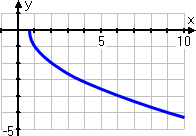
Now I'll do my graph:
Note that, since the domain starts at , the blue line of my graph could not go to the left of, nor below, the beginning point, . But the function continues forever in the other direction (that is, off to the upper right of my drawing area), so my graph needed to continue to the end of my drawing area on the top right-hand side of my picture.
Make sure you're careful about these domain and range issues for graphing with square roots.

-
Graph

As usual, I'll start by finding the domain. In order to do this, I have to solve the quadratic inside the square root; it may be easier just to look at (or think of) the graph of the quadratic.
Since the parabola is always above the x-axis, then x2 + 1 is always positive. Since the argument of the square root is always positive, then the values for x can be anything; there is no restriction on the domain of this particular square-root function.
If I have to "show my work" for the domain, then I would show that the inequality has a solution of "all real numbers":
x2 + 1 ≥ 0
x2 ≥ −1
Since any squared value is going to be zero or greater, then x2 will certainly always be greater than −1, for all x.
Continuing on, I do my T-chart. In this case, setting the argument of the square root equal to a perfect square number did not work out nicely, so I gave up and used decimal approximations from my calculator for plotting my points. I've listed the y-values accurate to three decimal places, which is more than sufficient for graphing purposes.
Finally, I'll do my graph:
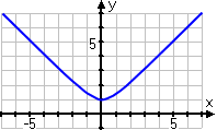
Please take particular note of the fact that, unlike an absolute-value graph, this graph does not have a sharp turn (that is, an "elbow") at the bottom; the turn is gently curved. Don't go too quickly when graphing with square roots; take the time to notice details like this.
© 2024 Purplemath, Inc. All right reserved. Web Design by ![]()