


Exponential Functions: Compound Interest
Purplemath
What is compound interest?
Compound (or compounded) interest is interest that is earned on interest. If you invest $300 in a compound-interest fund for two years at 10% interest annually, you will earn $30 for the first year, but then you will earn 10% of $330 (or $33) for the second year, for a total of $63 in interest.
The same investment in a simple-interest fund would earn 10% of the initial investment amount for each year; in other words, simple interest would be $30 a year, period. So you'd have just $60 in interest at the end of the two years.
What is the compound-interest formula?
One very important exponential equation is the compound-interest formula, which looks like this:
...where A is the ending amount, P is the beginning amount (or "principal"), r is the interest rate (expressed as a decimal), n is the number of compoundings a year, and t is the total number of years.
Regarding the variables in the compound-interest formula, the n refers to the number of compoundings in any one year, not to the total number of compoundings over the life of the investment. If interest is compounded yearly, then n = 1; if semi-annually, then n = 2; quarterly, then n = 4; monthly, then n = 12; weekly, then n = 52; daily, then n = 365; and so forth, regardless of the number of years involved.
Also, the value of "t" must be expressed in years, because interest rates are expressed that way (unless you're dealing with a loan-shark). If an exercise states that the principal was invested for six months, you would need to convert this to years; if it was invested for 15 months, then years; if it was invested for 90 days, then of a year; and so on.
(And, yes, you'll want to leave the fraction in exact form when you're doing your computations, because the decimal approximation can create severe round-off errors with exponentials. Wait to round until the end, when you're at the end of your final computation with a given input value.)
Note that, for any given interest rate, the above formula can be simplified to the simpler exponential form that we're accustomed to. For instance, let the interest rate r be 3%, compounded monthly, and let the initial investment amount be $1250. Then the compound-interest equation, for an investment period of t years, becomes:
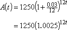
...where the base is 1.0025 and the exponent is the linear expression 12t.
To do compound-interest word problems, generally the only hard part is figuring out which values go where in the compound-interest formula. Once you have all the values plugged in properly, you can solve for whichever variable is left.
What is an example of using the compound-interest formula?
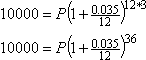
- Suppose that you expect to need $10,000 in thirty-six months' time when your teenager starts attending university. You plan to invest in an instrument yielding 3.5% interest, compounded monthly. How much should you invest?
To solve this, I have to figure out which values go with which variables. In this case, I want to end up with $10,000, so A = 10,000. The interest rate is 3.5%, so, expressed as a decimal, r = 0.035. The time-frame is thirty-six months, so years. And the interest is compounded monthly, so n = 12.
The only remaining variable is P, which stands for how much I will have started with. Since I am trying to figure out how much to invest in the first place, then solving for P makes sense.
I will plug in all the known values, and then simplify my equation:
Now I need to solve for the remaining variable.
The temptation at this point is to simplify on the right-hand side, and then divide off to solve for P. Don't do that; it tends toward round-off error, and can get you in trouble later on. Instead, stay exact, and do the dividing off symbolically (and exactly) first:
Now I'll do the whole simplification in my calculator, working from the inside out, so everything is carried in memory (in my calculator's "Ans" variable) and I get as exact an answer as possible:
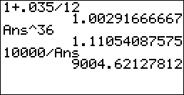
Rounding to dollars-and-cents (that is, rounding to two decimal places), I see that I need to invest:
about $9004.62
(The above exercise did not specify how to round my answer, but in this case it didn't need to. You always round dollars-and-cents values to two decimal places.)

Should I memorize the compound-interest formula?
You should memorize the compound-interest formula, but you should also memorize the meaning of each of the variables in the formula. While you might be given the formula on the test, it is unlikely that you will be given the meanings of the variables, and, without the meanings, you will not be able to complete the exercises.
© 2024 Purplemath, Inc. All right reserved. Web Design by ![]()